My Laptop Has an Unused NPU. I Want to Finally Find Out Whether It Can Be Useful
My Lenovo Yoga Slim 7x has another processor alongside the usual CPU and GPU: an NPU (Neural Processing Unit), designed to run neural network computations in an energy-efficient way. In everyday use, apart from things like blurring the background during calls or indexing files in the background, it mostly sits idle. I decided to check what else I could do with it, how fast it is, and whether it is worth using in practice.
I started by checking which language models I could run on it, which tools I needed, and how much work the setup took. I measured generation speed, response latency, the effects of context settings and input length, and behavior on battery. I did not obtain reliable RAM measurements or evaluate response quality.
I hope a local LLM will be useful when the connection to the cloud is poor or unavailable, for example on a plane or a train. It might be enough to help with text, code, or notes stored on the laptop. It is also useful to know which tasks I can handle without sending a prompt to an external model. An NPU could be particularly useful here: it was designed to run neural networks using less energy than a CPU or GPU, and ASUS explicitly connects NPUs with lower power consumption and longer battery life (ASUS). I compared speed and collected preliminary power readings, but did not measure battery runtime.
I did not assume that a local model would replace the cloud, or that the NPU had to beat the CPU or GPU. The experiment explored when it is worth using the NPU, which execution path to choose, and where its practical usefulness ends. Finding scenarios where the CPU or GPU was more practical was a useful result too.
Another motivation is simply to learn more about the technology and experiment with model settings.
The starting point was Qwen3-4B-Instruct-2507. I tested F16, Q8_0, Q4_K_M, and Q4_0 GGUF variants and a prepared W4A16 QNN package, then compared Qwen3 sizes from 1.7B to 32B on the CPU. I also varied context window capacities and actual input lengths. All comparisons ran on native Windows ARM64 on this laptop.
Key results:
- Short input, AC power: the CPU with Q4_0 gives about 33 tokens/s - the fastest.
- Battery + Power Saving: the NPU (qairt) maintained about 20 tokens/s, making it my starting point for responsive use in this mode.
- Long input (6180 tokens): about 33 s on the NPU versus about 86 s on the CPU.
- Model size: 8B and 14B offered usable interactive speeds; I found 32B (about 4.8 tokens/s) too slow for comfortable interactive chat in this test.
- The NPU is not automatically the best choice - it depends on the scenario.
The power figures in the chart below are approximate net SYS readings from separate single-run measurements, with responses of different lengths and content. Counter coverage and measurement error have not been established. These are not measurements of battery runtime or energy for an identical task.
Longer input can change which device is faster. With 420 input tokens, the CPU finished generation sooner: 6.69 s versus 9.31 s on the NPU. With 6180 input tokens, the NPU took 32.96 s and the CPU 86.03 s - the NPU was about 2.6× faster in this test.
1. Background
1.1. Hardware
I’m testing a Yoga Slim 7x with a Snapdragon X Elite X1E-78-100 and 32 GB of RAM. There are three compute devices within this single SoC that can run model computations.
The laptop has a Qualcomm Snapdragon X Elite with three compute units:
- CPU - 12 Qualcomm Oryon cores, split into three clusters of four, running at up to 3.4 GHz under multicore workloads.
- GPU - integrated Qualcomm Adreno X1-85, using shared RAM, with OpenCL support.
- NPU - Qualcomm Hexagon, rated at up to 45 TOPS (trillion operations per second).
TFLOPS and TOPS don’t translate directly into tokens/s. Generation speed also depends on the model, data transfers from memory, and the compute implementation. It needs to be measured for a specific configuration.
1.2. Models and Files
Models Used
In the tests, I mainly used Qwen3-4B-Instruct-2507. The 4B in its name means approximately four billion parameters. This version only operates in non-thinking mode. A smaller model is not just a more heavily quantized version of a larger one. It has a different parameter count, and individual models can also differ in architecture and training.
For comparison, I also measured Qwen3-1.7B, 8B, 14B, and 32B on the CPU with thinking disabled.
I also tried running Qwen3-235B-A22B Q4_K_M, a Mixture of Experts (MoE) model. In this architecture, a router selects a subset of experts to process each token. The 235B-A22B label means about 235 billion parameters in total and about 22 billion active when processing a token. It does not mean that memory for just 22B worth of weights will be enough. In my test, the model did not finish loading, so I have no speed result for it.
Model File Formats
Models are stored in different formats. These can differ in both the contents and the number of files, even for the same model. This is why a model such as Qwen can be downloaded in several versions. The main formats and their differences are described below.
PyTorch Weight Files
Older Hugging Face repositories often contain files such as pytorch_model.bin, as well as files with .pt and .pth extensions, saved using PyTorch’s serialization mechanism. Under the hood, this uses Python’s pickle module. Because loading pickle data can execute malicious code, this format is being replaced by safer alternatives.
Safetensors
This format was created to address the security problems associated with pickle-based weight files. A .safetensors file is a flat binary buffer containing tensor names, types, dimensions, and values. It works well for safely sharing model weights, but does not store the complete computational architecture of the model.
GGUF
GGML is a tensor computation library used by llama.cpp, among other tools. GGUF is a model file format from this ecosystem. It can contain not only weights, including quantized weights, but also extensible metadata: the architecture name, its parameters, the tokenizer, and the chat template.
QNN Contexts and DLC
Instead of giving a program just the weights, we can prepare the computations for an accelerator ahead of time. Qualcomm’s tools take a network description and its weights, transform the computations into a form supported by the selected backend, and allow the result to be saved. This saved representation is a QNN context.
In packages for Hexagon chips, the context is often split into .bin files. These are a completely different format from the PyTorch .bin files described above. .DLC (Deep Learning Container) is Qualcomm’s dedicated container for storing a network, and can also contain a prepared context.
How Does the Program Know How to Build the Network from These Files?
This depends on the format and the ecosystem used to run the model:
- Hugging Face (Safetensors / PyTorch): The weight files provide the numbers. A typical repository also includes a
config.jsonfile specifying the architecture type and its parameters, such as the number of layers and vector dimensions. The code implementing that architecture usually comes from the externaltransformerslibrary. A class such asAutoModelForCausalLMreads the configuration, which might point toQwen3ForCausalLM, creates the network structure, and then loads the weights into it. The tokenizer is supplied in separate files. - GGML (GGUF): The architecture code does not come from Transformers. It is built into the program, such as
llama.cpp. The program reads the GGUF file to identify the architecture, for example Qwen3, retrieves the network settings stored in the container, and uses its own implementation to set up the computations (Qwen3 implementation in llama.cpp). Supporting a new architecture therefore requires updating the program itself, not just converting the weights to GGUF. - Qualcomm (QNN/DLC): The program loads ready-made, precompiled instructions for the accelerator through the QNN execution interface. It does not need to build the architecture layer by layer and assign weights as Transformers or llama.cpp does. This typically requires the prepared
.bincontexts, package configuration, and tokenizer.
ONNX: A Computation Graph and Its Execution
ONNX, or Open Neural Network Exchange, was created as a common model representation for moving models between tools. It is not a library that runs the model. It describes computations independently of a particular hardware implementation.
An ONNX model contains:
- operations and the connections between them,
- inputs and outputs, their types and dimensions, and the versions of the operator sets used,
- weights and constants, or references to separate data files.
A simple example:
x → MatMul with W → Add b → Relu → ySafetensors can store W and b. An ONNX file contains the structure of the whole graph, its inputs and outputs, and the weights themselves. The runtime still needs to know how to execute MatMul, Add, and Relu.
ONNX describes a graph that the runtime uses to prepare execution. In ONNX Runtime, the simplified process looks like this:
- Optimization: ORT loads the graph and simplifies it in software, for example by precomputing constant parts or combining adjacent operations into a faster one.
- It divides the work between Execution Providers, which integrate backends and accelerators. For example, on Snapdragon I am interested in the QNN Execution Provider.
- The provider prepares the supported parts for its backend, and the runtime coordinates execution. Operations can run through existing kernels or a prepared engine, rather than by directly executing ONNX instructions.
Unsupported operations can fall back to the CPU if the configuration allows it. Otherwise, execution may be rejected.
File Format Summary
| File / format | Contents | Typical software | Where do computations run? |
|---|---|---|---|
.safetensors |
Named tensors, their types, dimensions, and values. Also quantized representations, if supported by the tool | PyTorch + Transformers; an external library supplies the architecture code | On devices supported by the software stack. The format alone does not provide an NPU execution path on my Yoga |
pytorch_model.bin |
Objects saved using PyTorch serialization (pickle) | PyTorch or a library built on it | Depends on the PyTorch implementation and backends |
.gguf |
Model tensors and metadata, optionally the tokenizer and chat template | llama.cpp | CPU, GPU, or NPU, if the build and backend support the model and tensor types |
.onnx |
A hardware-independent operation graph and its associated weights | ONNX Runtime (ORT) | CPU, GPU, or NPU through the appropriate Execution Provider. Not every graph runs on every device |
QNN context .bin |
Opaque, compiled instructions for specific hardware | QNN interface, for example through the qairt plugin |
In the path discussed here, the HTP backend and Hexagon NPU |
.dlc |
Deep Learning Container: Qualcomm’s network container, which can also include a prepared context | Compatible Qualcomm tools and runtime | Requires strict compatibility between the file, target SoC, and software version |
1.3. What Can Run the Model on the CPU, GPU, and NPU?
Running a model on specific hardware requires a runtime to load the model and coordinate execution, and a compute backend to execute supported operations on the device.
llama.cpp
This runtime reads GGUF files. It implements supported model architectures and delegates work to compute backends. On this platform, I’m interested in three of them: CPU, OpenCL for the Adreno GPU, and the experimental ggml-hexagon for the Hexagon NPU.
Qualcomm’s ecosystem has its own terminology for the different layers of the stack:
| Name | Role |
|---|---|
| QNN | Low-level API and backend layer for compiling and executing graphs |
| QNN HTP backend | QNN backend that sends supported computations to Hexagon. HTP stands for Hexagon Tensor Processor |
| QAIRT | Qualcomm’s broader SDK and runtime tool stack |
| Genie | Generative framework within Qualcomm’s ecosystem |
| GenieX | Tools and SDK offering flexible execution paths, including a plugin system |
| ONNX Runtime GenAI | A higher-level layer based on ONNX Runtime, handling the token generation loop, sampling, and KV cache, among other things |
GenieX
This is Qualcomm’s plugin-based tool for running models. Its plugins include llama_cpp for GGUF files and qairt for prepared QNN packages. I measured both paths. Qualcomm describes GenieX as a community edition of Genie, but the names are not interchangeable. Genie handles generation in other integrations, for example the NPU model path in AnythingLLM, where the application downloads a package containing a Genie configuration and precompiled QNN files.
I ran the speed tests through GenieX. Although I also tried a standalone llama.cpp build during setup, the results later in this article come from GenieX. I did not benchmark the Genie integration within ORT.
Execution Paths and Hardware Summary
| Model artifact | Software / integration | Path to the device |
|---|---|---|
| GGUF | Standalone llama.cpp or GenieX with the llama_cpp plugin |
CPU backend → Oryon cores |
| GGUF | Standalone llama.cpp or GenieX with the llama_cpp plugin |
OpenCL backend → Adreno GPU |
| GGUF | Standalone llama.cpp or GenieX with the llama_cpp plugin |
ggml-hexagon → Hexagon NPU |
| QNN context package | GenieX with the qairt plugin |
QNN → HTP backend → Hexagon NPU |
| ONNX model prepared for QNN | ONNX Runtime GenAI with QNN EP | QNN → HTP backend → Hexagon NPU |
| Package compatible with ORT’s Genie path | ORT GenAI with the Genie backend | Qualcomm stack → Hexagon NPU |
These paths are described in more detail in the GenieX documentation and the ORT GenAI guide to QNN and Genie.
Running a GGUF model on Hexagon does not require converting it to ONNX or going through QNN first. Conversely, two other paths sharing QNN does not guarantee identical speed or interchangeable packages.
The CPU controls the NPU, handles text tokenization, and performs sampling. This is expected and is not the same as model computations falling back from the accelerator to the CPU.
1.4. Quantization
Quantization approximates numerical values using a limited representation. Fewer bits can mean a smaller file, lower memory use, and less data to transfer. It does not guarantee a speedup: the backend needs an efficient implementation of the scheme. It can also change the model’s responses.
| Label | What does it mean? |
|---|---|
| BF16 / F16 | No quantization (16-bit). Full weights. BF16 preserves a wider numerical range at the expense of fractional precision; F16 makes the opposite trade-off |
| Q8_0 | 8-bit block quantization in GGML. Blocks of weights are approximated by 8-bit integer codes and a shared scale, rather than simply truncating each original weight to 8 bits |
| Q4_0 | 4-bit block quantization in GGML. Weights are approximated by 4-bit codes with shared scales. This reduces storage and can affect response quality, but that effect was not measured here |
| Q4_K_M | Mixed-precision block quantization in GGML. It combines Q4_K with higher precision for selected tensors, including Q6_K. It may offer a different size, speed, and quality trade-off from Q4_0, but I did not establish the best variant for quality here |
| W4A16 (in QNN) |
A precision label, not a file format. Qualcomm’s recipe nominally uses INT4 weights (W - Weights) and INT16 activations (A - Activations), not FP16 activations. It is not a strict equivalent of a single GGML format |
I did not evaluate response quality, so these labels and speed results do not establish a quality ranking or an optimal size-to-quality trade-off.
What Does “4-Bit” Quantization Mean in Practice?
It does not mean that each original weight is stored as a separate, precise number taking exactly 4 bits. In block quantization, we store an approximation using a short code and a scale, which lets us reconstruct an approximate value on the fly. Four bits alone provide just 16 possible values.
In Q4_0, weights are grouped into blocks of 32. Each block shares one 16-bit scale:
One Q4_0 block:
[ scale: 2 bytes ] + [ 32 codes of 4 bits each: 16 bytes ]

Total: 18 bytes for 32 weights.
This averages 4.5 bits per model parameter.
The scale and codes work together. “Q4” describes a specific block structure, not an idealized 4 bits of memory for every individual weight.
W4A16: Weights Are Not the Only Numbers in the Network
During inference, two different types of data appear in memory:
- Weights (W): the learned model parameters. They are static and are only read during text generation.
- Activations (A): temporary computation results passed between layers. They change with each input being processed.
A simplified view is: input activations × weights → output activations.
W4A16 is a precision label, not a file format.
In Qualcomm’s recipe, it nominally means INT4 integer weights and INT16 activations, not floating-point FP16. The label describes the intended numerical precision, but does not define the block layout as Q4_0 does, the KV cache precision, or how the NPU accumulates results. Although Q4_0 and W4A16 both have a four in the name, they describe different quantization schemes at different levels of abstraction.
What Am I Actually Comparing?
I’m checking what is worth running on this laptop’s CPU, GPU, and NPU, with which quantization, and under which conditions. The NPU was the starting point, but I don’t assume it will be the best choice. I ran the measurements through GenieX:
| GenieX path | Device or mode | Tested 4B variants |
|---|---|---|
llama_cpp |
CPU | GGUF: F16, Q8_0, Q4_K_M, Q4_0 |
llama_cpp + OpenCL |
Adreno GPU | GGUF Q4_0 |
llama_cpp + ggml-hexagon |
Hexagon NPU | GGUF: F16, Q8_0, Q4_K_M, Q4_0 |
llama_cpp, hybrid mode |
Mixed mode, without a verified breakdown of the work | GGUF Q4_0 |
qairt + QNN HTP |
Hexagon NPU | Prepared QNN W4A16 package |
Separately, I tested models from 1.7B to 32B on the CPU, larger context window capacities, and longer inputs. I also compared behavior on AC power, battery, and with Power Saving enabled.
When comparing the same GGUF across devices, I keep the model file unchanged. Switching to a QNN package also changes the quantization and runtime, so that result compares complete configurations, not just hardware.
1.5. Reading the Timing, Context, and Memory Results
- Prefill: processing the input.
- TTFT: time from the start of a request to the first response token.
- Decode: the rate of generating subsequent tokens, in tokens/s.
Reported TTFT and generation times do not include loading the model. A shorter TTFT does not necessarily mean the full response finishes sooner.
Window capacity is not input length. The input, history, chat markers, and response share the context budget. The KV cache stores part of the computations for retained tokens, but a longer history still increases memory and attention costs. This is why I vary window capacity and actual prompt length separately.
Model file size is not the same as RAM use. There are also caches, activations, buffers, and memory used by the system. I did not obtain reliable RAM measurements.
2. What Actually Ran
First, I checked whether each environment could initialize the model and generate a response at all. Only stable, working configurations made it into the final performance measurements.
2.1. Environment Summary
| Environment | Local test result | Benchmark included? |
|---|---|---|
| Standalone llama.cpp (ARM64) | CPU works, and OpenCL correctly detects Adreno. The ggml-hexagon build detects the NPU but cannot open a session |
No |
GenieX + llama_cpp |
Generation works in all modes: CPU, GPU, NPU, and hybrid | Yes |
GenieX + qairt |
The precompiled QNN package (W4A16) loads and runs on the NPU | Yes |
| ONNX Runtime GenAI | A potential alternative, but without a successfully completed local generation test | No |
Setup and Problems
Standalone llama.cpp
The ARM64 build for the CPU compiled successfully and runs reliably. The version with the ggml-hexagon backend detects the NPU, but loading the model fails when it tries to open a session. I have not established the cause. This does not show that the hardware cannot run the model: the same compute path worked through the llama.cpp libraries included with GenieX.
GenieX with the llama_cpp Plugin (GGUF)
I registered a local GGUF file and tested NPU initialization. The performance measurements covered CPU, GPU, NPU, and hybrid modes. In hybrid mode, the actual distribution of work between the SoC’s compute units remains a black box from the user’s perspective.
GenieX with the qairt Plugin (QNN Package)
I used a prepared QNN W4A16 package for Snapdragon X Elite chips, compatible with the qairt plugin.
2.2. What I Did Not Measure
I considered ORT as an alternative, but testing it would require preparing or obtaining a compatible model, configuring generation, and verifying the selected integration. That would be a separate stage of work requiring more time. I therefore limited the scope to working GenieX configurations. The lack of ORT results is a scope decision, not evidence that this path does not work.
3. How I Measure and What I Compare
I tested GenieX v0.10.0 with QAIRT 2.50 and its bundled llama.cpp version.
I ran the speed measurements natively on Windows ARM64 through GenieX. For the speed and quantization tables, each completed cell consists of one warm-up run and five measured runs. I report the median. Window capacity and input length tests have three measured runs each. Settings are a limit of 128 new tokens, non-thinking mode, temperature 0, and seed 42. In the baseline 4B comparison, llama_cpp used a 512-token window, while qairt used the package configuration. The separate input length series use a fixed 16,384-token window.
Each run is the first request in a new process. A warm-up run may warm the system and file cache, but not the runtime instance used by the next run. Reported generation times exclude loading the model. The same prompt text produces 48 input tokens in llama_cpp and 61 in qairt. The two paths use different artifacts and configurations, so the TTFT comparison does not isolate the effect of hardware.
I set the power states manually: AC power, battery, and battery with Power Saving.
4. Results: Speed, Energy, and Input Length
The charts show results from recorded runs. Error bars on the speed charts show the minimum and maximum, not a confidence interval. AC means connected to the charger, and Power Saving means the energy-saving mode.
4.1. Speed: 4B in Three Power States
Medians from five runs after one warm-up run. The exception is the CPU with Power Saving, where the warm-up run timed out. The response limit is 128 tokens, with thinking disabled. The llama_cpp window is 512 tokens; the qairt window comes from the package.
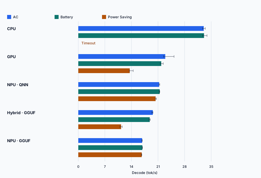
| Path | Decode on AC (tokens/s) | Decode on battery (tokens/s) | Decode on battery + Power Saving (tokens/s) |
|---|---|---|---|
| llama_cpp CPU | 33.0 | 33.1 | ⏱ timeout |
| llama_cpp GPU (Adreno) | 22.9 | 21.8 | 13.6 |
| GenieX qairt (QNN → NPU) | 21.3 | 21.4 | 20.4 |
| llama_cpp hybrid | 19.6 | 18.8 | 11.3 |
| llama_cpp NPU (ggml-hexagon) | 16.8 | 16.9 | 16.7 |
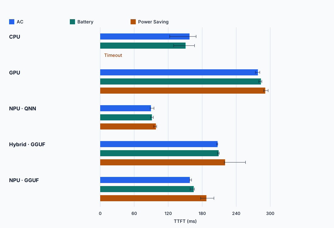
qairt had the shortest TTFT: medians of 89–98 ms depending on the power state. The CPU achieved 150–158 ms, the NPU through ggml-hexagon 158–187 ms, hybrid 207–220 ms, and the GPU 278–291 ms. These are results for complete execution paths, not the devices alone: qairt processed 61 input tokens, while llama_cpp processed 48.
4.2. Average Power: How Many Watts Did the Measurement Show?
To make the comparison easier to read, I show average net power in watts (W). Watts describe how quickly energy is being used, not how much energy the entire response consumed. Lower power does not always mean less energy per task if the model has to run much longer.
These are estimates from the SYS channel after subtracting a separately measured idle baseline. They are not the laptop’s total wall power or a measurement of the NPU alone. I calculated the average from the recorded energy and elapsed run time, including model loading. Historical readings from the two series required different unit conversions. The exact counter coverage and measurement error have not been established.
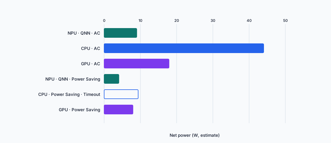
| Configuration | Average net SYS power, W ≈ | Run time, s | Response tokens |
|---|---|---|---|
| qairt, AC | 9.0 | 96 | 1563 |
| CPU, AC | 44.0 | 62 | 1448 |
| GPU, AC | 17.9 | 96 | 2048 |
| qairt, battery + Power Saving | 4.1 | 117 | 1563 |
| GPU, battery + Power Saving | 7.9 | 201 | 2048 |
| CPU, battery + Power Saving, timeout | 9.4 | 1802 | No completed result |
In simple terms: in a separate AC-powered run, the readings were about 44 W for the CPU, 18 W for the GPU, and 9 W for qairt on the NPU. On battery with Power Saving, qairt showed about 4 W and the GPU about 8 W. This looks promising for the NPU, but it is not a battery life prediction.
There is only one run per configuration, and the responses differ in both length and content. I therefore do not treat these numbers as the cost of performing an identical task. The CPU timeout is a separate observation, not a completed test. The battery series changes both the power source and the operating mode, so it does not isolate the effect of Power Saving alone.
4.3. What Would I Choose on Battery and with Power Saving?
Unplugging the charger alone did not change speed much in this short test: decode differed by less than 1% for the CPU and both NPU paths, about 4.6% for the GPU, and 4.1% for hybrid.
With Power Saving, I would choose the NPU for its tested speed and responsiveness. qairt maintained about 20.4 tokens/s, and ggml-hexagon 16.7 tokens/s. The GPU dropped to 13.6 tokens/s, hybrid to 11.3 tokens/s, and the CPU did not finish the warm-up within the 15-minute limit. During that run, I observed activity on 8 of the 12 threads, but did not establish the cause of the delay.
The NPU was therefore my preferred tested path for responsive use in this mode, but not the only one that worked: the GPU still generated text. The separate lower approximate SYS power reading for qairt is preliminary supporting evidence, not proof that it provides the longest battery runtime.
4.4. Quantization: 4B on CPU and NPU through ggml-hexagon
AC power, a short prompt, medians from five runs. The chart shows decode: the rate of generating subsequent tokens.
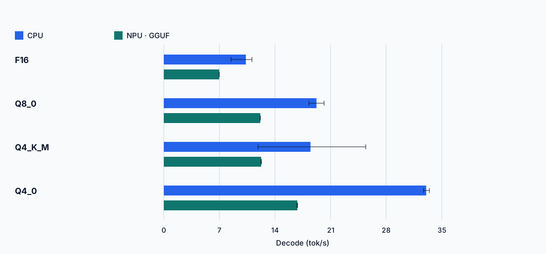
| Quantization | CPU | NPU (ggml-hexagon) |
|---|---|---|
| F16 | 10.3 | 7.0 |
| Q8_0 | 19.2 | 12.1 |
| Q4_K_M | 18.5 | 12.3 |
| Q4_0 | 33.0 | 16.8 |
The separate qairt QNN W4A16 package achieved 21.3 tokens/s. I do not include it in the same GGUF quantization series.
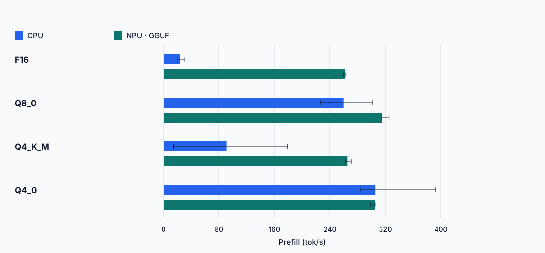
On the CPU, Q4_0 was about 3.2 times faster than F16 in decode and more than 12 times faster in prefill. The NPU had slower decode for all these GGUF variants, but smaller prefill differences between quantization schemes. This is a result for this model and build, not a general ranking of the schemes. This series measured speed, not response quality.
4.5. Parameter Count: From 1.7B to 32B on the CPU
AC power, Q4_K_M, non-thinking, five measured runs each.
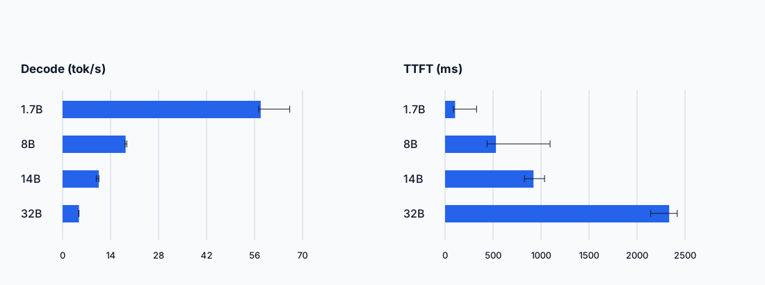
| Parameters | Decode (tokens/s) | Prefill (tokens/s) | TTFT (ms) |
|---|---|---|---|
| 1.7B | 57.8 | 500.4 | 104 |
| 8B | 18.4 | 98.3 | 530 |
| 14B | 10.5 | 56.5 | 921 |
| 32B | 4.8 | 22.3 | 2335 |
- These are original Qwen3 models with switchable thinking/non-thinking modes, tested here with thinking disabled. The 4B-2507 model is a different checkpoint, so it does not belong directly in this series.
Which of These Are Practical?
- 1.7B: the most speed headroom. A useful starting point for simple, narrow tasks, but check whether the quality is enough.
- 8B: about 18 tokens/s with a short input is a reasonable starting point for interactive work.
- 14B: about 10.5 tokens/s. Slower, but still a reasonable option if the larger model gives a better result for a particular task.
- 32B: about 4.8 tokens/s. Decoding 128 tokens alone takes roughly 27 seconds: too slow for comfortable interactive chat in this test. It could still be useful for batch tasks if waiting is acceptable, but its quality for those tasks needs assessment; I did not measure it.
32B is the largest model for which I obtained a result in this series, not an established limit of this laptop. These runs use short inputs and a 512-token window. Speed does not demonstrate quality, and a longer document could change responsiveness considerably.
4.6. Window Capacity and Actual Input Length
Changing Window Capacity with a Short Prompt (CPU, AC)
I varied the window capacity while keeping 52 input tokens and 128 response tokens. The history therefore grew to about 180 positions, not 65k or 262k. Below are median TTFT values from three runs per cell.
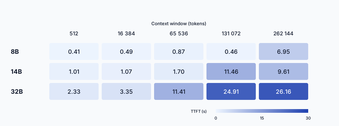
| Parameters | 512 | 16,384 | 65,536 | 131,072 | 262,144 |
|---|---|---|---|---|---|
| 8B | 0.41 s | 0.49 s | 0.87 s | 0.46 s | 6.95 s |
| 14B | 1.01 s | 1.07 s | 1.70 s | 11.46 s | 9.61 s |
| 32B | 2.33 s | 3.35 s | 11.41 s | 24.91 s | 26.16 s |
TTFT increased at larger limits, but not monotonically. I did not establish the cause or a practical document length limit: this test did not fill the window.
Longer Inputs with a Fixed Window (4B Q4_0, CPU and NPU)
On AC power with the maximum performance profile, I kept the window at 16,384 tokens and increased the length of a synthetic input made of repeated paragraphs. I ran the CPU series first, then the NPU through GenieX llama_cpp, meaning ggml-hexagon, not qairt. I used the same registered Qwen3-4B-Instruct-2507 Q4_0, identical prompts, temperature 0, and three measured runs per cell after one warm-up run. Each run used a new process, and each response had exactly 128 reported tokens and stopped at the length limit.
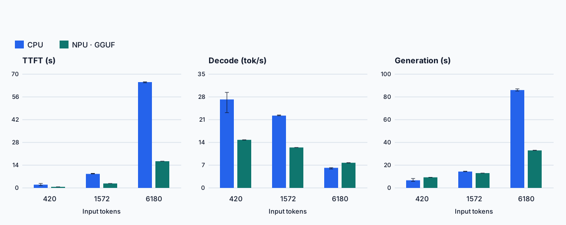
| Input tokens | CPU TTFT | NPU TTFT | CPU decode, tokens/s | NPU decode, tokens/s | CPU total generation | NPU total generation |
|---|---|---|---|---|---|---|
| 420 | 1.99 s | 0.66 s | 27.22 | 14.79 | 6.69 s | 9.31 s |
| 1572 | 8.63 s | 2.72 s | 22.25 | 12.44 | 14.38 s | 13.02 s |
| 6180 | 65.12 s | 16.42 s | 6.18 | 7.74 | 86.03 s | 32.96 s |
Total generation is the median of the engine-reported total generation time, excluding model loading, not the sum of medians for other metrics. CPU prefill was 211.2, 182.1, and 94.9 tokens/s respectively; NPU prefill was 640.9, 577.1, and 376.4 tokens/s.
With longer inputs, the NPU can be faster than the CPU. For 6180 input tokens and 128 response tokens, generation took about 33 seconds on the NPU versus 86 seconds on the CPU. With the shortest input, the CPU finished first. The choice therefore also depends on input and response length.
These are two separate findings: I measured the speed advantage for longer inputs through ggml-hexagon, and lower power in another series through qairt. I did not measure power or energy for this longer-input test.
Between the shortest and longest inputs, CPU decode dropped by about 77% and NPU decode by 48%. I do not attribute the drop to a single mechanism: the input is synthetic, the series ran from shortest to longest, and I did not record temperature or clock speeds. I did not measure energy or document task quality here.
5. What to Choose for a Particular Use Case
5.1. Practical Conclusions from These Tests
I would not pick one configuration for everything. First, I would decide whether response speed, battery use, document length, or the capabilities of a larger model matter most. The suggestions below are starting points for your own tasks, not a model quality ranking or a guarantee of how every application will behave.
| What you need | Starting point | What the tests confirm |
|---|---|---|
| Fast generation with a short input on AC power | 4B Q4_0 through GenieX llama_cpp on the CPU |
About 33 tokens/s. In a separate run, the CPU had higher average net power than qairt |
| Responsive use with Power Saving on battery | NPU: GenieX qairt, or alternatively llama_cpp |
20.4 and 16.7 tokens/s respectively. A separate preliminary reading showed about 4 W average net SYS power for qairt, not a measured battery-runtime advantage |
| A larger model for interactive work | Start with 8B or 14B Q4_K_M on the CPU | About 18.4 and 10.5 tokens/s with a short input. Evaluate quality on your own task |
| A longer input and short response | llama_cpp on the NPU |
With 6180 input tokens and 128 output tokens, about 33 seconds of generation versus 86 seconds on the CPU |
5.2. My Takeaways
The NPU turned out to be useful, and I will keep experimenting with it. It is not automatically the best choice just because it was designed for neural network computations:
- Short input and AC power: the CPU with Q4_0 gave the highest decode throughput for the tested 4B model. I don’t need to force the NPU into the workflow for a quick response.
- Power Saving: the NPU maintained responsiveness better than the GPU and hybrid mode. That tested speed makes
qairtmy first candidate in this mode; the separate lower SYS power reading remains preliminary, rather than evidence of longer battery life. - Longer input: ggml-hexagon could beat the CPU on total response time. A short-question benchmark is not enough to choose a configuration for documents.
- Model size: 8B and 14B look reasonable in terms of speed. 32B (about 4.8 tokens/s) was too slow for comfortable interactive chat in this test, but could still be useful for batch tasks if waiting is acceptable. Whether more parameters improve the result needs a task-specific quality assessment, which I did not perform.
The next step is to check whether the selected models actually handle real tasks well: editing text, summarizing notes, extracting information from documents, or helping with code.
I also want to see how to turn these working configurations into everyday use, for example in LM Studio, Ollama, or AnythingLLM.
LLMs are not the only possible use for the NPU. Audio transcription and image processing are other directions to explore, with different models and requirements.
P.S. A note on the language: this time I decided to try something new and wrote the article in Polish, my native language. I can put the text together faster and make fewer mistakes that way. LLMs seem to be very good at translation, so I used one to translate it into English. I’m curious to see how well this works.