Bielik on the Arduino VENTUNO Q NPU (Compared with Snapdragon X Elite)

1. Arduino VENTUNO Q

Alongside my laptop with its unused NPU, I also have an Arduino VENTUNO Q: a board with a Qualcomm Dragonwing IQ-8275, 16 GB of RAM, and a Hexagon NPU. It is time to take a closer look at this one too. In my previous experiment with a Snapdragon X Elite laptop, I checked what the laptop’s NPU could be useful for. Now I want to see what it offers on a smaller device: how large a model I can run and whether it responds fast enough.

A note on language: I am continuing an approach I tried in the previous article: writing in Polish and using an LLM to help translate the text into English. Polish is my native language, so I can write faster and make fewer mistakes that way. I was happy with how the translation turned out last time, so I am trying it again here. I review the English version afterwards, checking that it preserves the meaning and technical details of the original. As a bonus, I can publish the article in both languages.

I chose Bielik because I am interested in working in Polish, and this family of models was developed with that language in mind. The v3.0 series also lets me compare several sizes: 1.5B, 4.5B, and 11B. I tried Minitron 7B separately, outside the main comparison.

I deliberately chose v3.0 rather than the newer v3.1: v3.1 comes in one size (11B), and I did not even know whether that would run on the board’s NPU. With several v3.0 sizes, it was easier to find the practical boundary.

I wanted to answer three questions:

1. How large a Bielik model can I run, and how fast does it respond?
2. How does quantization affect results on selected Polish-language tasks?
3. How do I prepare my own model file when there is no ready-made GGUF?

Key results: The laptop’s CPU generated tokens faster than its NPU, but the board told a different story.

• On VENTUNO Q, Bielik 4.5B Q4_0 in npu mode achieved 11.5 tokens/s, compared with 5.4 tokens/s on the CPU. Time to first token was about 0.46 s instead of 4.53 s.
• On X Elite, the same 4.5B variant generated faster on the CPU: 28.2 versus 14.0 tokens/s.
• I could not run 11B on the board’s NPU: Q4_0 and Q4_K_M failed to load in npu and hybrid modes. The CPU worked, but managed only about 2.1-2.4 tokens/s.
• Q8_0 changed the results on the selected Polish-language tasks only slightly. Q4_0 had a larger effect that varied by task.

2. Which Bielik, and How Do the Versions Differ?

2.1. A Family of Models, Not One File

Bielik is a family of language models developed by SpeakLeash in collaboration with ACK Cyfronet AGH. Their training data includes Polish, but the models are not limited to Polish. In this experiment, I used the v3.0-Instruct variants, fine-tuned to follow instructions and hold conversations. The v3.0 models tested here are released under Apache 2.0.

Name	What it means in this article
Bielik-1.5B-v3.0-Instruct	The smallest model tested, with about 1.6 billion parameters
Bielik-4.5B-v3.0-Instruct	The larger model in the Small series, with about 4.8 billion parameters
Bielik-Minitron-7B-v3.0-Instruct	A compressed version of 11B, with about 7.4-7.5 billion parameters - outside the main benchmark
Bielik-11B-v3.0-Instruct	The largest model in this comparison, with about 11.2 billion parameters

Minitron is not just a more heavily quantized 11B. It was produced through structural pruning and knowledge distillation: the network itself changes, not just the precision used to store its numbers. The Bielik-Minitron-7B report describes the details.

Base variants are base models, before instruction tuning. Here I test Instruct. The family name is no substitute for checking the version and license of a particular model.

For running the models, the important point is that llama.cpp supports them. 11B has 50 layers and a declared context window of 32,768 tokens. The Small series has an 8192-token window. Small is not simply a scaled-down copy of 11B: its architecture and training differ, even though both series declare the LlamaForCausalLM class. The llama label in the metadata does not mean I downloaded an unmodified Llama model from Meta. The Bielik 11B v3 and Bielik Small reports explain the details.

2.2. What I Am Not Testing Here

• v3.1: the official series includes only a standalone 11B model. v3.0 let me compare several sizes. I do not apply the v3.0 results to the newer version.
• DFlash: an auxiliary model for speeding up generation through speculative decoding, not a small, standalone replacement for 11B.
• FP8 and AWQ: other ways of preparing weights. Here I compare GGUF in Q4_0, Q8_0, and Q4_K_M, not every available format.
• Bielik-PL-11B and PL-Minitron-7B: separate variants, outside this article’s results.

3. How Does the Model Reach the NPU?

A model can run as GGUF through the Hexagon backend, or be prepared with Qualcomm’s tools for execution through QNN. QNN can also be used by ONNX Runtime through the QNN Execution Provider, which officially supports inference on Linux ARM64.

Here I test GGUF. I have not yet tested compiling Bielik for QNN and running it through a plugin such as qairt, or running it through ONNX Runtime on VENTUNO Q.

I used GenieX, Qualcomm’s tool with several execution plugins. The one used in this article is llama_cpp:

GGUF -> GenieX, plugin llama_cpp -> backend ggml-hexagon -> Hexagon NPU

This is not the compiled QNN graph path. It does not require exporting the model to ONNX first.

Why did I start with Q4_0? The Arduino tutorial explicitly recommends it for the NPU: “For NPU execution, prefer a Q4_0 quantization”. I also tested Q8_0 and Q4_K_M.

4. How and Where I Tested

4.1. Hardware and Speed Measurements

Component	Laptop	Board
Device	Lenovo Yoga Slim 7x	Arduino VENTUNO Q
SoC	Snapdragon X Elite X1E-78-100	Dragonwing IQ-8275
Hexagon	HTP v73	HTP v75
RAM	32 GB	16 GB
OS	Windows ARM64	Ubuntu 24.04 ARM64
GenieX	v0.10.0	v0.9.3

The main comparison covers 1.5B, 4.5B, and 11B, Q4_0, Q8_0, and Q4_K_M quantizations, and cpu, npu, and hybrid modes. I did not test 11B Q8_0 on the board because of the problems described later.

Each complete series includes a warm-up run and five measured runs. I report the median of five runs from the last complete series for each configuration. I do not mix these with individual startup tests or calculate a median of medians from different sessions.

Settings: a 4096-token window, a limit of 128 new tokens, seed 42, and --think=false. The effective temperature was 0.8: the plugin replaced the requested 0 with its default. TTFT is the engine-reported time to first token, excluding model loading. Prefill means processing the question, and decode means generating the answer.

I used the same prompt in every run. I kept the test prompt in Polish:

Wyjaśnij po polsku, czym różnią się CPU, GPU i NPU podczas lokalnego uruchamiania dużych modeli językowych. Opisz kolejno przetwarzanie promptu, generowanie kolejnych tokenów, pamięć wag i pamięć roboczą oraz znaczenie opóźnienia pierwszego tokenu. Użyj kilku pełnych akapitów, podaj przykład asystenta głosowego i zakończ krótkim podsumowaniem. Nie skracaj odpowiedzi do listy haseł.

4.2. How I Evaluated Quality

I compared F16/BF16, Q4_0, and Q8_0 on 5174 examples from five tasks used by the Open PL LLM Leaderboard, following the SpeakLeash task definitions. I ran the multiple-choice tests through llama-server on an RTX 4090 with CUDA under Linux, using 0-shot evaluation without a chat template. This does not measure free-form conversation quality or the correctness of NPU execution.

5. Results

5.1. X Elite: The CPU Generates Faster, the NPU Starts Sooner

I compared 27 combinations of these three models, three quantizations, and three modes. The table shows generation throughput (decode), in tokens/s.

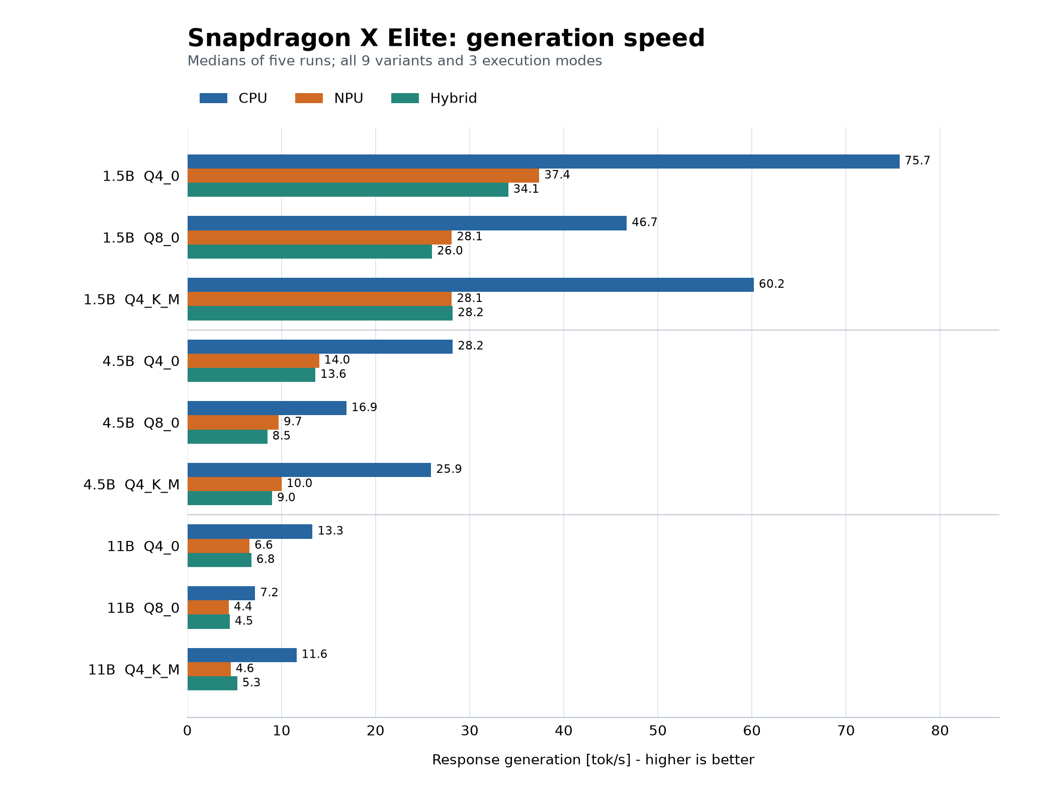
Model	Quantization	CPU	NPU	Hybrid
1.5B	Q4_0	75.7	37.4	34.1
1.5B	Q8_0	46.7	28.1	26.0
1.5B	Q4_K_M	60.2	28.1	28.2
4.5B	Q4_0	28.2	14.0	13.6
4.5B	Q8_0	16.9	9.7	8.5
4.5B	Q4_K_M	25.9	10.0	9.0
11B	Q4_0	13.3	6.6	6.8
11B	Q8_0	7.2	4.4	4.5
11B	Q4_K_M	11.6	4.6	5.3

The CPU won on decode in all these configurations. For 11B Q4_0, it was about twice as fast as NPU mode. That does not mean the NPU lost at every stage of the response. For Q4_0:

Model	CPU TTFT	NPU TTFT	CPU prefill	NPU prefill
1.5B	142 ms	131 ms	749 tokens/s	810 tokens/s
4.5B	473 ms	319 ms	224 tokens/s	333 tokens/s
11B	1492 ms	732 ms	108 tokens/s	220 tokens/s

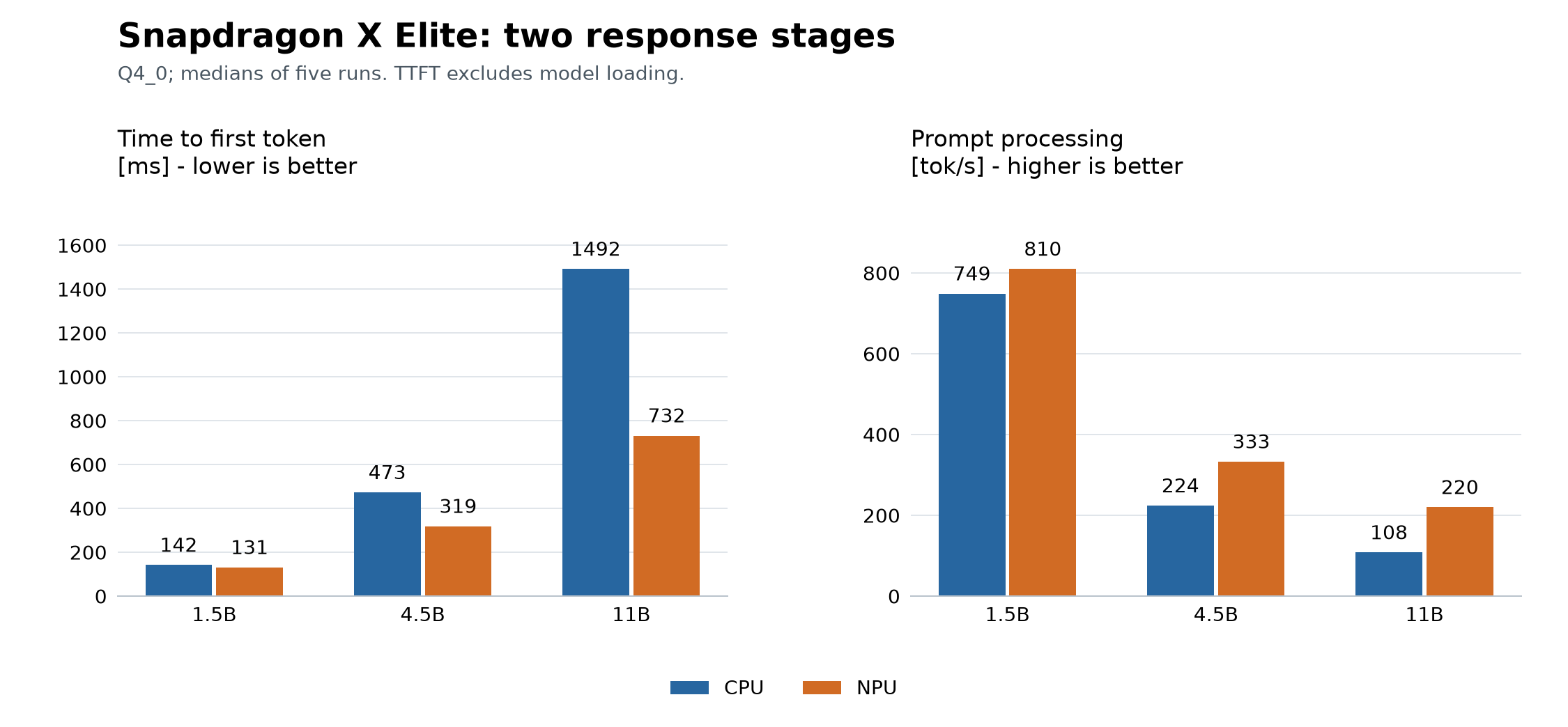
The NPU processed the input faster. The choice also depends on whether I am waiting for the response to start or for it to finish. With this short input and a longer response, the CPU’s higher decode throughput worked in its favor. I did not test a series of long documents, which could change the balance.

hybrid did not beat the CPU on decode.

5.2. VENTUNO Q: The NPU Makes a Practical Difference

On the board, the balance shifted. For working configurations, the numbers below are decode tokens/s / prefill tokens/s / TTFT ms, in that order. Each value is the median of five runs.

Model	Quantization	NPU	CPU	Hybrid
1.5B	Q4_0	29.1 / 657 / 162	15.9* / 76.5 / 1385	13.8 / 138 / 767
1.5B	Q8_0	19.7 / 618 / 172	9.7 / 56 / 1886	9.7 / 134 / 792
1.5B	Q4_K_M	24.5 / 626 / 170	12.3 / 40 / 2666	6.0 / 89 / 1193
4.5B	Q4_0	11.5 / 233 / 456	5.4 / 23 / 4534	5.5 / 51 / 2071
4.5B	Q8_0	Load failed	3.2 / 16 / 6498	Load failed
4.5B	Q4_K_M	9.2 / 244 / 437	5.0 / 12 / 8751	2.9 / 32 / 3316
11B	Q4_0	Load failed	2.4 / 12 / 13236	Load failed
11B	Q4_K_M	Load failed	2.1 / 5.7 / 28488	Load failed

The most interesting result for me is 4.5B Q4_0. The NPU generated about 2.1 times faster than the CPU, and the first token arrived about ten times sooner. Q4_K_M also worked, but decode was 9.2 rather than 11.5 tokens/s. For 1.5B Q8_0 and Q4_K_M, the NPU was about twice as fast as the CPU on decode.

That still does not mean the board beat the laptop. On the laptop, 4.5B Q4_0 on the CPU managed 28.2 tokens/s. The main lesson is which mode to choose on a particular device, not that a newer Hexagon is automatically faster at everything.

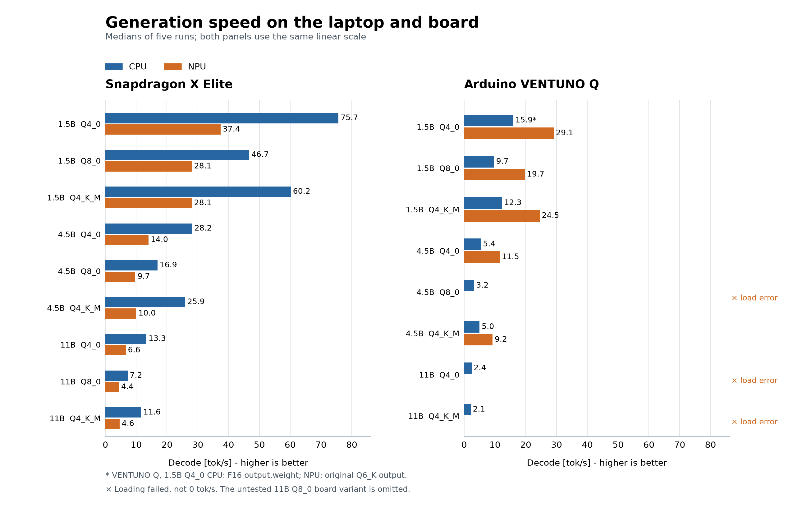*Medians from five runs. Crosses indicate loading failures, not zero throughput. 11B Q8_0 was not tested on the board. The asterisk beside 1.5B CPU marks a repeated measurement with the output tensor kept in F16.*

5.3. Why Did the Larger Models Fail to Load?

Model	Quantization	File size	NPU test on VENTUNO Q
1.5B	Q4_0 / Q8_0 / Q4_K_M	About 0.9 / 1.7 / 1.0 GB	Generation worked
4.5B	Q4_0 / Q4_K_M	2.70 / 2.88 GB	Generation worked
4.5B	Q8_0	5.06 GB	Load failed
11B	Q4_0 / Q4_K_M	About 6.3 / 6.7 GB	Load failed

The largest variant that loaded was 4.5B Q4_K_M (2.88 GB). The smallest that failed was 4.5B Q8_0 (5.06 GB).

The failures shared a signature, for example with 4.5B Q8_0:

ggml-hex: HTP0 buffer mapping failed : domain_id 3 size 58068992 fd 80 error 0x00000001
ggml-hex: fastrpc_mmap failed
SDKError(Model loading failed)

FastRPC handles communication between the host and DSP and the mapping of shared buffers. This log says that a buffer could not be mapped while loading the model. The 58 068 992 bytes refer to one buffer, not the whole model or the amount of free memory.

The Hexagon backend documentation describes a roughly 3.5 GB, 32-bit virtual address window per session. This is not the maximum GGUF file size. The same document explains how dynamically mapping and unmapping weights allows a larger model to run in a single session. The KV cache, which stores attention keys and values for context tokens, and active buffers also occupy address space.

Additional diagnostics of the shared backend path showed a failed host-side IOVA address allocation and propagation of ENOMEM to FastRPC.

The most likely explanation for the failures with larger variants is therefore a problem allocating address space for device mappings. Dynamic weight mapping was not enough to run the larger tested variants in this configuration. I did not establish a fixed GGUF size limit, or determine whether address allocation failed because of occupied address space, fragmentation, alignment requirements, or the way mappings were kept alive.

Offloading only some layers to the NPU, or using another backend version, remain possible ways to look for a workaround. The Qualcomm documentation also describes splitting the graph. Whether this path will run Bielik 11B on VENTUNO Q still needs to be tested.

5.4. What Is the Cost of Quantization?

Below are changes in accuracy relative to F16 for 1.5B/4.5B and BF16 for 11B, in percentage points. A minus means a lower score than the reference. A plus means a higher score on this dataset. Each precision was evaluated on the same 5174 examples.

Model	Quantization	polemo2_in	polemo2_out	klej_ner	cbd	belebele
1.5B	Q4_0	-3.9	-4.0	+2.2	+0.4	-2.4
1.5B	Q8_0	+0.8	-0.4	-0.8	+0.1	+0.4
4.5B	Q4_0	-2.4	-7.5	+5.5	-2.8	+0.3
4.5B	Q8_0	+2.5	+1.8	-1.1	-0.2	-0.2
11B	Q4_0	-0.7	-1.2	+0.6	+3.1	-0.2
11B	Q8_0	-0.1	+0.6	-0.2	+0.1	-0.2

The chart shows the absolute Belebele score, a reading comprehension task: 900 questions in the Polish version. This is a broader language task, better suited to an overall comparison than a single sentiment test or named-entity category task.

Model	F16/BF16	Q4_0	Q8_0
1.5B	60.6	58.1	61.0
4.5B	77.8	78.1	77.6
11B	86.1	85.9	85.9

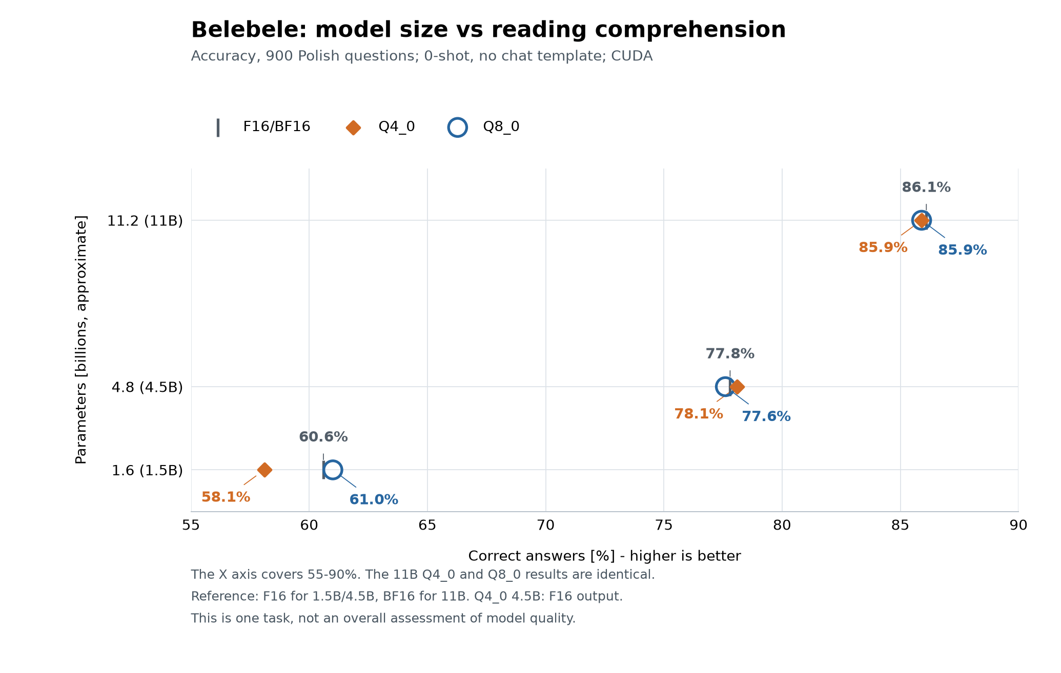
In this task, the differences between model sizes are larger than those between the tested weight precisions: 4.5B Q4_0 clearly outperforms 1.5B F16, while 11B Q4_0 stays close to its BF16 reference. That does not mean quantization is equally forgiving on every task, as the table of changes above shows.

These results describe resilience to quantization, not the model’s overall quality. Q8_0 stayed close to the reference: differences did not exceed about 2.5 percentage points, and were usually less than 1 percentage point. Q4_0 changed the scores more, and unevenly: 4.5B lost 7.5 percentage points on polemo2_out, but gained 5.5 on klej_ner.

Why are there gains after reducing precision? Quantization changes the scores assigned to possible answers. If two answers have similar scores, even a small change can flip the choice: sometimes to a wrong answer, sometimes to a correct one. There is no guarantee that accuracy will fall on every task. This does not prove that the lower-precision model has become better overall. I also do not treat every small difference as a meaningful improvement or loss.

These numbers answer the question: how did scores on selected tasks change after quantization under a fixed evaluation method? They do not test free-form conversation, the grammar of generated text, tool calling, or the correctness of NPU computations. I did not evaluate Q4_K_M quality here.

5.5. Same File, Different Results: One Token on the CPU, a Full Response on the NPU

I ran into an interesting bug while testing 1.5B Q4_0 quantization. The same GGUF file behaved differently across configurations:

• Board CPU: one token, for example “O”, followed by EOS - the end-of-sequence marker.
• Board NPU: 128 response tokens, reaching the configured limit.
• Laptop and desktop CPUs: generation without this premature termination.

I found a practical workaround in the quantization settings: keeping output.weight in F16 with --leave-output-tensor removed the symptom in the CPU runs I performed. This matrix turns the model’s state into scores for all tokens in the vocabulary, including EOS, so changing its precision can change the next token selected. For this 1.5B tensor, keeping F16 instead of Q6_K increased weight storage by about 55.3 MiB.

6. How to Prepare GGUF Files and Their Quantizations

Preparation has two steps: saving the weights in GGUF and reducing their precision through quantization. I use tools from llama.cpp. The examples below assume the converter’s dependencies are installed and llama-quantize has been built.

6.1. From Hugging Face Weights to GGUF

The llama.cpp converter rewrites a model from Hugging Face format to GGUF: it reads the configuration, tokenizer, and all weight shards, then saves them in the format used by llama.cpp. If I already have a GGUF file, conversion is unnecessary. The downloaded model directory must contain the weights, configuration, and tokenizer. Exporting 11B to BF16:

python3 llama.cpp/convert_hf_to_gguf.py models/Bielik-11B-v3.0-Instruct \
  --outfile Bielik-11B.bf16.gguf --outtype bf16

6.2. From GGUF to Q4_0, Q8_0, and Q4_K_M

llama-quantize takes the source file, output filename, and quantization type:

./llama.cpp/build/bin/llama-quantize Bielik-11B.bf16.gguf Bielik-11B.Q4_0.gguf Q4_0
./llama.cpp/build/bin/llama-quantize Bielik-11B.bf16.gguf Bielik-11B.Q8_0.gguf Q8_0
./llama.cpp/build/bin/llama-quantize Bielik-11B.bf16.gguf Bielik-11B.Q4_K_M.gguf Q4_K_M

To keep the output tensor at its original precision:

./llama.cpp/build/bin/llama-quantize --leave-output-tensor \
  Bielik-11B.bf16.gguf Bielik-11B.Q4_0-lo.gguf Q4_0

This is the option that removed premature EOS for 1.5B on the board’s CPU (§5.5). The Q4_0 label alone does not mean every tensor uses four bits. The quantizer documentation describes the syntax and options.

6.3. Running through GenieX

For the test on the board, I choose the working 4.5B Q4_0 variant. I register the model directory and run GenieX v0.9.3:

geniex pull local/bielik-4p5b-q4_0 \
  --model-hub localfs --local-path /home/arduino/bielik/4.5b/q4_0 \
  --model-type llm --skip-update

geniex infer local/bielik-4p5b-q4_0 \
  --compute npu --nctx 4096 --max-tokens 128 --think=false \
  --temperature 0.8 --seed 42 --input prompt.txt \
  --verbose --log info --skip-update

Changing --compute npu to --compute cpu lets me test the same file on the CPU. The Arduino tutorial covers installing GenieX.

7. Summary

Getting a model to run is not enough. It also needs to run fast enough to be useful. I used a working threshold of TTFT up to 3 s and decode of at least 8 tokens/s.

Need	My starting point	Why
Assistant on VENTUNO Q	4.5B Q4_0 on the NPU	The largest model that ran at a practical speed
A larger Bielik on the laptop	11B Q4_0 on the CPU	The largest available Bielik - ~13.3 tokens/s
More speed headroom on the board	1.5B Q4_0 on the NPU	~29.1 tokens/s - a small model to check on the intended tasks

On the board, I would choose the NPU. On the laptop, not necessarily. For the working 1.5B and 4.5B variants, the board’s NPU offered a practical advantage. On X Elite, the CPU generated subsequent tokens faster. The RTX 4090 served as the common backend for quality evaluation, not as a participant in the speed comparison between these devices. There is no universal “the NPU always wins” - the result depends on the model, device, and software.

Running a larger Bielik remains a problem. The tested 11B variants did not finish loading in npu and hybrid modes on the board. I recorded a FastRPC mapping error. Diagnostics of the shared path point to a failed host-side IOVA address allocation (§5.3). This does not prove that the hardware can never run such a model, or that QNN necessarily has to be the solution.

The next step is to check the selected configuration on real assistant tasks. Further FastRPC diagnosis, QNN compilation, audio, and integration with Home Assistant remain separate stages.

I am publishing ready-made Q4_0 variants on Hugging Face: Bielik-4.5B-v3.0-Instruct-GGUF-Q4_0 and Bielik-11B-v3.0-Instruct-GGUF-Q4_0.